Introduction to Design Patterns

What is a Design Pattern?

Design patterns represent solutions to common problems in software design. They are like blueprints that work as high level design methodologies for your software. A pattern is not a specific piece of code like a library or an algorithm, but a general concept that you can follow. While an algorithm is like a cooking recipe that has exact and clear steps, a design pattern is like a blueprint where you can see the overall picture and the outcome, but no specific steps to follow.

A pattern description mostly consists of the problem the pattern tries to solve, the solution, the structure of classes used for the solution and their relationships, and some code examples.

Most patterns emerged to solve problems in object-oriented design, but other patterns have emerged continuously.

Why is a pattern useful?

You can code without knowing a single design pattern, or you might be implementing some patterns without knowing it. However, knowing popular design patterns is useful because:

1. Design patterns are tried and tested solutions to common problems in software design. You can have solutions to all sorts of problems under your belt, using principles of object-oriented design.

2. Design patterns can be used as common language that you and your teammates can communicate around. When discussing problems, suggesting a design pattern as a solution will immediately make sense to everyone that knows about the pattern beforehand.

3. Optimal design pattern application prevents the need for refactoring code, as the application of the design pattern often is an already optimal solution.

4. Design patterns are built around object-oriented principles and strengthen their advantages, leading to cleaner code, less bugs through proper encapsulation etc, more intuitive interface to the client caller.

Criticism of patterns

• A workaround for a weak programming language - Sometimes, the need for patterns comes from using a programming language that lacks necessary featrues or levels of abstractions. For example, the Strategy pattern can be implemented with a simple anonymous (lambda) function in most modern programming languages. This means that sometimes it can be more inefficient to implement a pattern than to choose a language that already implements the pattern.

• Inefficient solutions - A pattern can lead to inefficient solutions, especially when they are implemented ‘exactly as the pattern is defined’, without adapting them to the specifc project context. Too much unnecessary overhead can thus occur.

• Unjustified use - Many novice programmers who have just learned about patterns may try to apply them everywhere, even in situations where simpler code would be better.

Pattern Types

By Complexity

Design patterns are very different in their complexity, level of detail, applicability to the entire system. An analogy for different design patterns is where in road construction, you can improve the safety of an intersection by, 1) installing some traffic lights, or 2) building an entire multi-level intersection with underground pedestrian passages.

The most basic and low-level patterns are called ‘idioms’, and are usually specific to a single programming language. Universal and high-level patterns are called architectural patterns, which can be implemented in any language. They are used to design the overall architecture of an entire application.

By Purpose

Design patterns can be categorized by their purpose, or role in the software. 3 main groups are:

1. Creational patterns: provide object creation mechanisms that increase code reusage and flexibility.

2. Structural patterns: Provde a way to assemble objects and classes into larger structures in a flexible, efficient manner

3. Behavioural patterns: Provide methods of effective communication and assignment of responsibilities between objects.

Reference:

• https://refactoring.guru/design-patterns
• https://dotnettekki.com/csharp-design-patterns/

B-tree & 인덱싱

데이터베이스의 성능을 개선하는 방법중에 가장 먼저 떠오르는 것은 단연 인덱스를 생성하는 것이다. 오늘은 인덱스의 내부 작동 원리에 대해 알아보려고 한다. 물론 각 데이터베이스마다 세부적인 방식에 차이가 있겠지만, 대표적으로 많이 쓰이는 인덱싱 방법인 B-tree에 대해서 알아보자.

B-tree란?

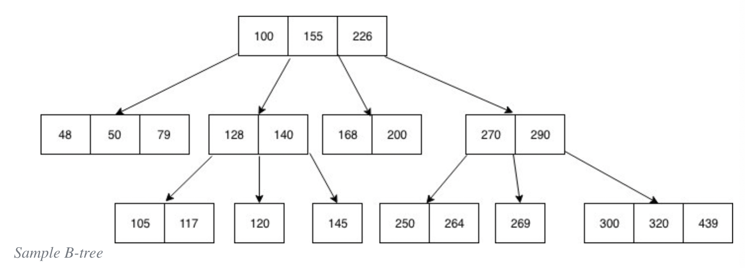
B-tree는 트리방식의 자료구조인데, 노드의 순서를 고려한 트리구조라고 보면 되겠다.

각 노드는 하나의 숫자키가 아닌 여러개의 숫자키를 담고 있는데, 특징을 보자면:

• 각 노드의 키는 오름차순으로 정렬되어 있다
• 각각의 키는 최대 포인터 두개를 가지고 있으며, 각 포인터는 하위 노드를 가리킨다
• 숫자키의 왼쪽 포인터가 가리키는 노드는 더 작은 숫자들로 이루어진 노드, 오른쪽 포인터가 가리키는 노드는 더 높은 숫자들로 이루어진 노드이다.
• 한 노드가 ‘n’개의 숫자키를 가지고 있다면, 포인터의 개수는 최대 ‘n+1’이 된다.

자, 그럼 이 b-tree가 데이터베이스에서 많이 사용되는 이유는 무엇일까?

데이터베이스는 말그대로 데이터를 저장하는 곳으로, 그 일을 잘 수행하기 위해서 b-tree라는 자료구조가 내부적으로 사용되어 진다.

b-tree를 잠시 잊고, array 즉 리스트라는 자료구조에 데이터를 저장한다고 생각해보자.

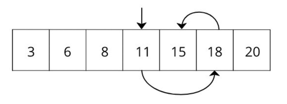
그 자료구조 즉 데이터베이스 테이블에 ‘15’라는 숫자가 들어있는지 확인하려면 어떻게 해야하는가?

만약 오름차순으로 정렬이 되어있지 않다면, 그냥 생으로 처음부터 한칸씩 열어보며 15가 있는지 없는지 확인을 할 수밖에 없다. 데이터의 숫자가 n일 때, O(n)이라는 성능이 나오게 된다.

만약 정렬이 되어있다면 조금 나을 것이다. 왜냐면 binary search라는 알고리즘을 사용해서 반씩 나누어서 찾다보면, O(log n)이라는 시간안에 해당 숫자를 (만약 있다면) 찾을 수 있기 때문이다.

즉, binary search를 이용하면 원래 5번 걸려서 찾을 것이 3번이면 된다.

B-tree의 가장 단순한 종류인 binary tree도 이런 원리를 사용해 트리화 한 것인데, 차이는 물리적으로 리스트 안에 자료를 저장하기 보다는 reference 포인터를 이용해서 자료가 있는 디스크의 주소를 가르킨다는 점이다.

이런 점은 자료를 쓰는 write 작업의 효율성을 높여주게 되는데, 정렬된 리스트 같은 경우 숫자를 중간에 집어넣는 write 작업이 O(n)인 반면 (옆에 숫자들을 다 옴겨서 자리를 만들어줘야 하므로), binary tree의 경우는 그냥 맞는 자리를 찾은다음 슥 넣어주기만 하면 되므로 대체적으로 O(log n)의 성능을 가지게 된다.

그리고 이런 binary tree를 좀더 여러개의 자료를 담을 수 있는 형태로 쪼개서 발전 시킨 것이 b-tree라고 보면 되겠다. (binary tree는 노드에 숫자 한개, 따라서 각 노드의 자식 노드의 개수도 두개뿐이지만 b-tree는 각 노드당 담을 수 있는 숫자도 여러개고 한 노드의 자식 노드도 여러개다).

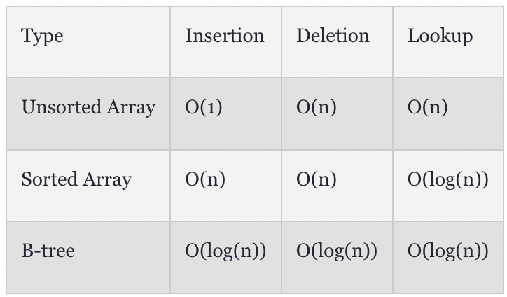
정리하자면 성능 차이는 아래와 같다.

자료의 읽고 쓰는 작업의 속도가 가장 중요한 데이터베이스가 b-tree 자료구조를 쓰는 이유이다.

(B-tree는 binary tree와 달리 두갈래가 아닌 여러갈래로 쪼개지므로 엄밀한 성능은 예를 들어 log4 n 이 되므로 binary tree보다도 성능이 좋을 것이다).

B+tree란?

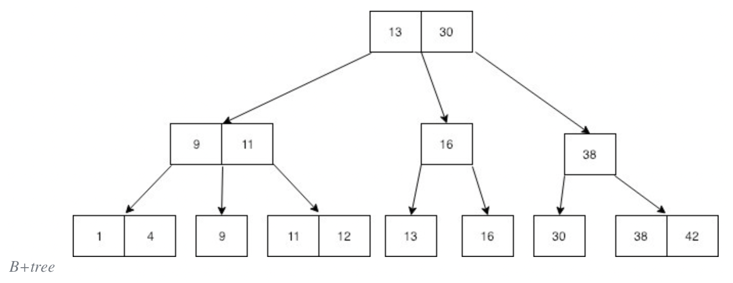
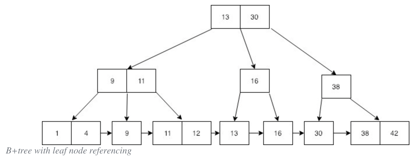
B+tree는 B-tree와 비슷한 자료구조로 B-tree와 상당히 비슷하게 생겼다. 차이점은 바로 모든 자료 즉 모든 숫자키가 가장 마지막 줄인 leaf 노드에 중복으로 들어간다는 점이다.

또한 모든 Leaf 노드는 오름차순으로 정렬되어 있는 것을 볼 수 있다. B+tree에서 leaf 노드들은 실제 ‘데이터가 저장되어지는 곳’으로 보면 되겠다.

추가적으로 만약 leaf 노드들 사이에도 추가 포인터들을 설치해준다면 순차적으로 모든 데이터를 순회하는 것 또한 가능하게 된다.

데이터베이스에 적용하기

위에 서술한 B-tree와 B+tree가 데이터베이스 인덱싱에 실제로 어떻게 사용되어지는지 보자.

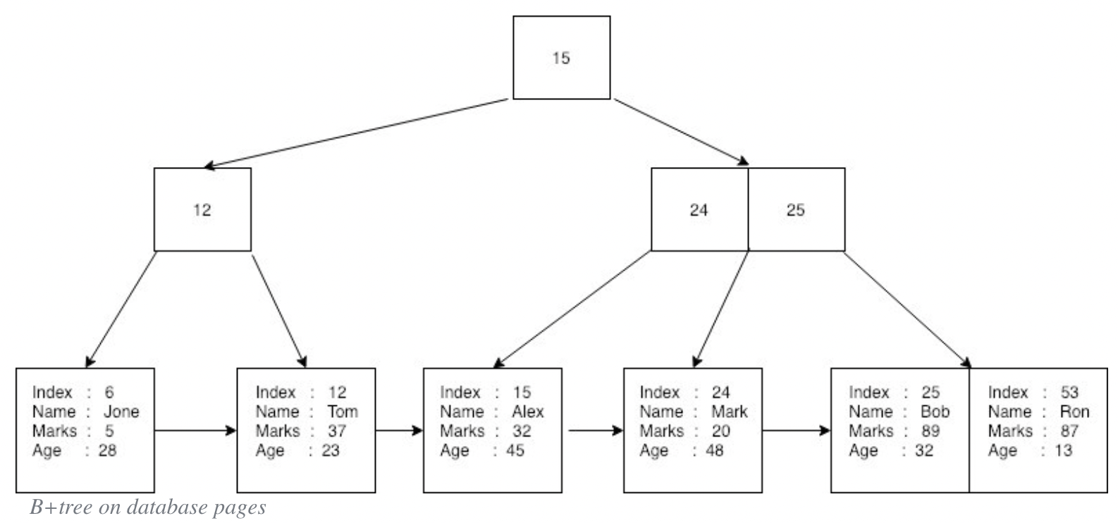
이런 테이블이 있다고 해보자.

이름, 성적, 나이라는 세가지 컬럼이 있다.

이 데이터는 b+tree에 이렇게 저장된다.

각 노드의 숫자는 각 데이터행의 primary key 가 되고, 맨 아래 leaf 노드들에 실제 데이터가 저장이 된다. 프라이머리 키로 데이터를 조회하고자 할 때 이런식의 데이터구조로 인해 빠른 조회가 가능하게 된다. 또한 각 데이터들도 오름차순으로 정렬이 되어있고 포인터가 존재하기 때문에, ‘key < 15’ 와 같은 범위적인 쿼리도 빨리 할 수 있고, 이름이 ‘Alex’ 인 사람을 찾는 것도 데이터를 순회하며 할 수 있다.

(테이블을 생성하면 기본적으로 primary key를기준으로 clustered index가 생성되는 것으로 알고 있는데, 이런 구조가 아닐까 싶다. 더 조사가 필요하다.)

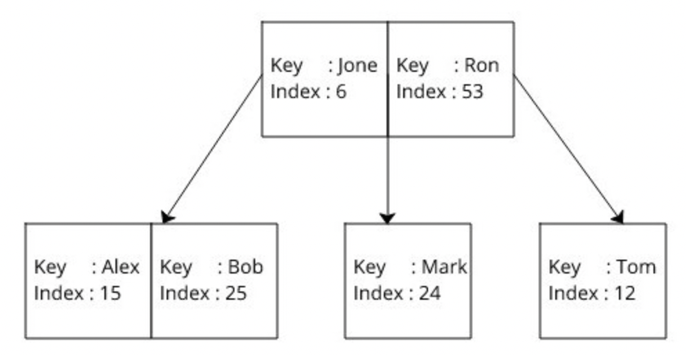
만약 프라이머리 키가 아닌 다른 값, 예를 들어 이름으로 조회 쿼리를 많이 한다고 한다면 ‘Name’ 컬럼에 인덱스를 매겨주는 것이 좋은 방법일 것이다. 이런 추가적 인덱스, 즉 non-clustered index는 b-tree에 생성이 된다.

각 노드는 key, value를 가지게 되는데 이 때 key는 인덱스 컬럼의 값 (이름) 그리고 value는 실제 데이터가 저장된 곳을 찾을 수 있는 값, 즉 프라이머리 키의 값이다. b-tree는 key를 기준으로 정렬이 된다.

만약 ‘Alex’라는 사람을 찾고자 한다면 이 B-tree에서 해당 노드를 찾아서 프라이머리 키 값을 조회한 후, 자료가 저장되어 있는 B+tree에서 해당 프라이머리 키 값을 사용해 나머지 데이터를 조회하면 되는 것이다. O(log n) 조회를 두번 해야 하기 때문에 바로 clustered index를 이용해 조회하는 것보단 약간 느릴 것을 예상할 수 있다.

이상으로 데이터베이스에서 쓰이는 자료구조인 B-tree와 B+tree에 대해서 알아보았다.

Reference: https://dzone.com/articles/database-btree-indexing-in-sqlite

Async Programming

Blocking vs Non-blocking

Blocking refers to operations that block further execution until that operation finishes. Non-blocking refers to code that doesn’t block execution.

In the given example, localStorage is a blocking operation as it stalls execution to read. On the other hand, fetch is a non-blocking operation as it does not stall alert(3) from execution.

// Blocking: 1,... 2
alert(1);
var value = localStorage.getItem('foo');
alert(2);

// Non-blocking: 1, 3,... 2
alert(1);
fetch('example.com').then(() => alert(2));
alert(3);

Blocking code normally happens on I/O operations, which rely on external data or response. An I/O task is a task which the CPU cannot perform on its own and must wait for an external components, such as a network response. Usually this involves waiting a long time, compared to the CPU speed, so it’s better to switch to another task while waiting.

Advantages

One advantage of non-blocking, asynchronous operations is that you can maximize the usage of a single CPU as well as memory. CPU can perform other tasks while waiting, and return to the previous task once the IO task is done.

Synchronous & blocking example

An example of synchronous, blocking operations is how some web servers like ones in Java or PHP handle IO or network requests.

If the code reads from a file or the database, your code “blocks” everything after it from executing. In that period, your machine is holding onto memory and processing time for a thread that isn’t doing anything.

One way to handle other requests while that thread is waiting is to spawn more threads to work on other requests, which requires more resources (memory), which is referred to as concurrency or parallelism, a concept distinct from asynchronous programming.

Asynchronous, non-blocking example

Asynchronous, non-blocking servers - like ones made in Node or FastAPI - only use one thread to service all requests. This means an instance of Node makes the most out of a single thread. The creators designed it with the premise that the I/O and network operations are the bottleneck.

So when requests arrive at the server, they are serviced one at a time.

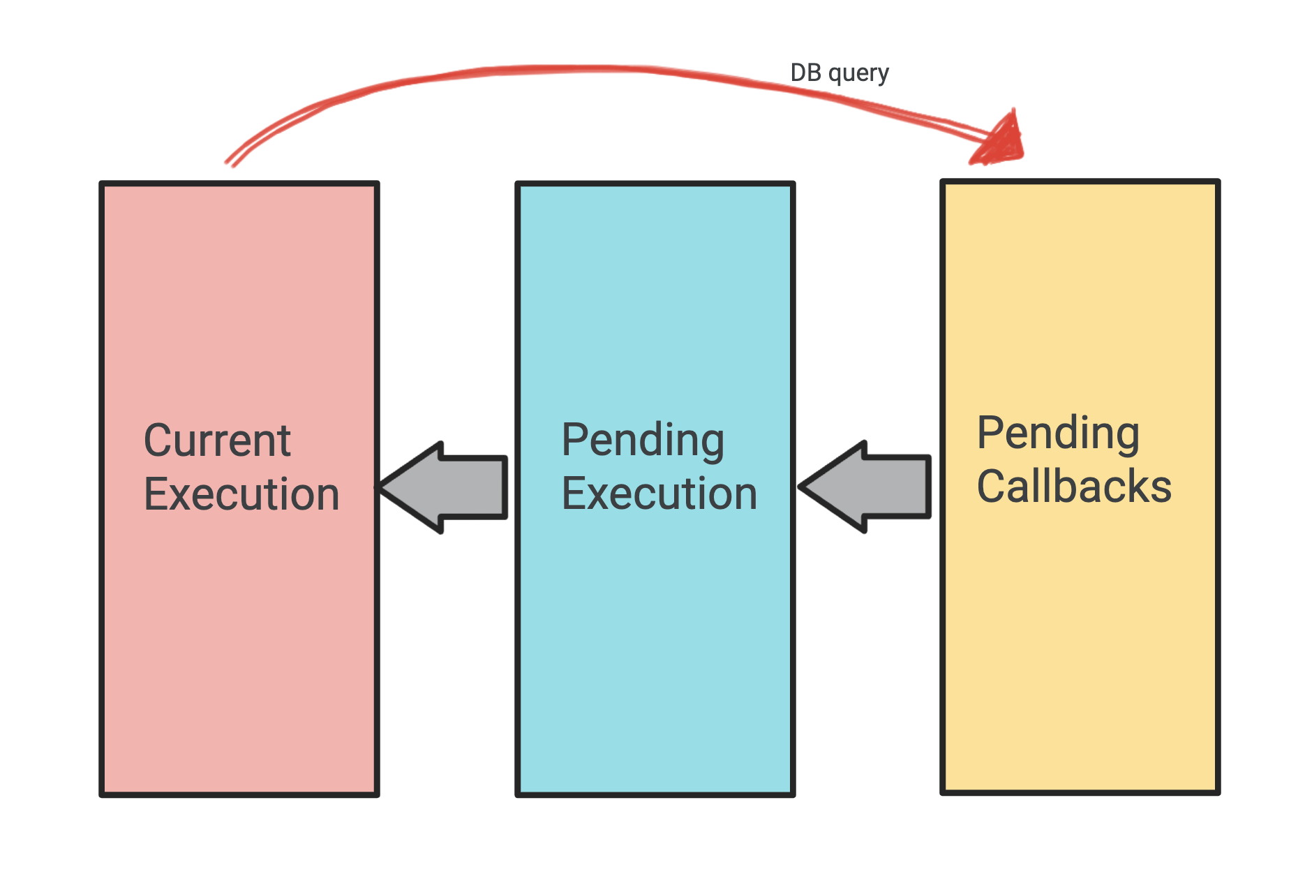
Picture 3 queues: The first queue is the current execution stack, second queue is for pending IO callbacks, and the third queue is tasks pending execution.

When the code needs to query the DB for example, it sends the callback to the second queue and the main thread will continue running (it doesn’t wait) on other tasks from the first and third queues. Now when the DB operation completes and returns, the corresponding callback is pulled out of the second queue and queued in the third queue. When the engine gets a chance to execute something else (current execution stack is empty), it picks up a callback from the third queue and executes it.

Performance

In pure terms, an asynchronous request is slower than an equivalent synchronous request because the thread works on other tasks before returning to the first task. However the real benefit happens when scalability is an issue, i.e. there are more requests than threads available. If there are 4 threads who are all working on potentially blocking IO requests, The remaining requests have to wait to even start.

The reason this is important is because in real world environments, it is impossible to correctly predict the load at any one time and have a server big enough to handle it using one thread per request. So it is important to maximise the server’s hardware capabilities to handle as many requests as possible, and an asynchronous server can handle several times the number of concurrent requests as a synchronous sever when both thread pools are at the max level.

Also, async code scales faster than synchrounous, because synchrounous code can’t scale faster than the thread injection rate. So a sudden heavy load means very slow response time.

It is important to note that async code does not completely replace the need for a thread pool (multiple threads). It’s not one or the other - async code allows the app to make optimum use of the thread pool, and draw out its maximum efficiency. So I guess it is always better to choose async over sync with scalability in mind.

Time Complexity (+ what does O(log n) mean?!)

Source: Big ‘O’ & Time Complexity

Time Complexity & Big O

Time complexity refers to how long an algorithm takes to run. The important thing here is it measures the run time of an algorithm respective to the input size.

Big O is a way to describe the speed of an algorithm as input size nears infinity (asymptotic analysis). The unit of measurement is the number of operations performed by the CPU, rather than the absolute time in seconds or minutes. One CPU operation refers to one read/write operation on a memory address, which is done in O(1) time.

In other words, Big O is a measure of scalability, i.e. how effective the algorithm is as input size increases massively.

The ‘O’ comes from ‘Order of the function’.

It’s important to note the importance of not only Time Complexity but also Space Complexity which is how much memory an algorithm consumes. This is also denoted by Big O.

Common Complexities

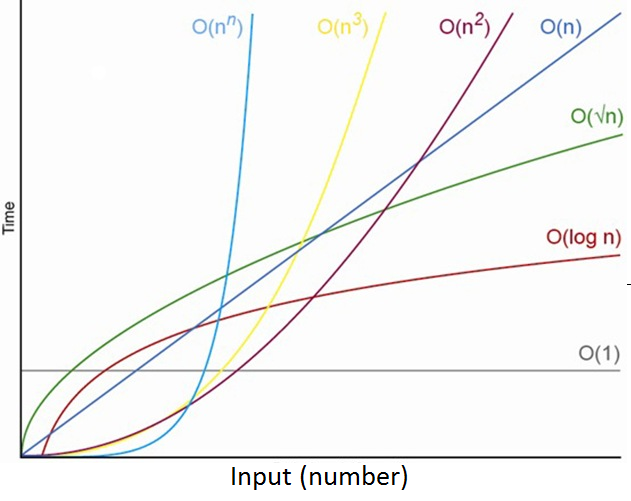
Common complexities in order from fast to slow are:

1. Constant: O(1)
2. Logarithmic: O(log n)
3. Linear: O(n)
4. Log-Linear: O(n log n)
5. Quadratic: O(n²)
6. Cubic: O(n³)
7. Exponential: O(2ⁿ)
8. Factorial: O(n!)

O(1) complexity means that an algorithm will always execute in the same amount of time regardless of input size. If it had 3 operations when n size was 1, it will still have 3 operations to complete when n size is 1,000,000.

Meanwhile, O(n) complexity denotes an algorithm whose number of operations grows linearly in direct proportion to the input data. For example, printing the elements of an array: If the array has 1 item print 1 item. If there are 1,000,000 items, need to print 1,000,000 times.

O(n²) complexity describes an algorithm whose performance is directly proportional to the square of the input size n. An example is nested for loops: if array size is 10, number of operations becomes 100. If n is 1,000, there will be 1,000,000 operations.

It is important to note that the complexity of an algorithm usually denotes the worst-case complexity, instead of the average case.

For example, some sorting algorithms have varying time complexities depending on how they are initially sorted. In such cases, they may have O(n log n) average run-time, and O(n²) worst case run-time, in which case the latter becomes the algorithm’s complexity.

O(log n)

Here, I want to talk about O(log n) just because I have found logarithms to be scary as someone who is not that fond of anything mathematics 😅.

O(log n) basically means that the time complexity of an algorithm is the Logarithm of input size n.

Logarithm is a mathematical concept widely used in CS, and is defined by the following equation.

log_b(x) = y if and only if b^y = x

In CS, the base is always 2 which represents a binary logarithm, so the equation becomes:

log(n) = y if and only if 2^y = n

Here, y is represents the time taken to run the algorithm while n represents input size.

The pattern goes as follows:

2⁰ = 1 ——> log(1) = 0

2¹ = 2 ——> log(2) = 1

2² = 4 ——> log(4) = 2

2³ = 8 ——> log(8) = 3

2⁴ = 16 ——> log(16) = 4

Here, the numbers 1, 2, 4, 8, 16... represents input size n while 0, 1, 2, 3, 4..., the log of these values, represents the complexity of the algorithm. We can see that as the size of n doubles, the log value (exponent of 2) increases by 1.

2^x = N ——> 2^x+1 = N * 2

This means that as N increases (doubles), the log value of N (log n) only increases by a small amount (1). 2²⁰ == 1M, while 2³⁰ == 1B, which is a huge difference but the log(n) difference is only 10.

This is why O(log n) algorithms are very efficient, only coming after O(1) but way more so than O(n). This is because when input size doubles, the number of CPU operations only increases by 1.

O(log n) algorithms

Logarithmic time complexity is typically seen in algorithms that repeatedly cut the input size in half until it reaches an answer. Examples are array binary search, or the binary search tree.

e.g. If the array size was 8 and a binary search was performed, it would be cut in half 3 times until the size was 1. (2³ = 8)

SOLID Principles

SOLID is a set of object oriented programming principles that helps make code more maintainable and flexible. The term was coined by ‘Uncle Bob’ Martin in 2000, who is also famous for ‘Clean Code’. These principles can be applied to any object oriented language.

Note: Python does not have inherent interfaces, so I have used Metaclasses to illustrate how interfaces work in Python.

SOLID stands for 5 principles:

1. Single Responsibility Principle
2. Open/Closed Principle
3. Liskov Substitution Principle
4. Interface Segregation Principle
5. Dependency Inversion Principle

Single Responsibility Principle

A class should have a single responsibility, meaning it should only have one reason to change.

Looking at the following example of a FacebookUser class, it has several functionalities such as adding friends, adding posts, and login.

class SNSUser:
    _friends = []
    _posts = []
    _logged_in = False


    def __init__(self, userName, SNSName):
        self._name = name
        self._sns_name = SNSName # 'facebook', 'instagram'

    def addFriend(newFriend):
        if self._sns_name = "Facebook":
            if newFriend not in self.__friends and len(self.__friends < 1000):
                self.__friends.append(newFriend)
        if self._sns_name = "Instagram":
            if newFriend not in self.__friends and len(self.__friends < 100000000):
                self.__friends.append(newFriend)

    def addPost(content):
        self.__posts.append(content)
    
    def LoginUser(self):
        # Login logic...
        self._logged_in = True

The class is responsible for logging in the user, which might seem like a good idea. But what happens if we want to change the loging logic, or another type of login method? We would need to modify the class to change the Login method or add another one. Changing existing code should be stayed away from as much as possible, and instead, code should be constructed in an extensible manner.

A better approach thus is to separate the login methods as a separate class that handles all login logic.

class LoginHandler():
    def login_user_with_password(user: User):
        return some_login_method(user)
    
    def login_user_with_fingerprint(user: User):
        return finger_login(user)

When login logic changes or another method needs to be added, only this class needs to be modified, reducing the risk of bugs.

Open/Closed Principle

Classes should be open for extension, but closed for modification.

This means classes should be extended to change functionality, instead of being modified.

If we look at the previous code example, we can see that the SNSUser class handles both Facebook and Instagram users in its logic.

class SNSUser:
    #...

    def addFriend(newFriend):
        if self._sns_name = "Facebook":
            if newFriend not in self.__friends and len(self.__friends < 1000):
                self.__friends.append(newFriend)
        if self._sns_name = "Instagram":
            if newFriend not in self.__friends and len(self.__friends < 100000000):
                self.__friends.append(newFriend)
    #...

The class is checking if the current User’s SNS type is Facebook or Instagram, and adding friends accordingly.

The problem with this setup is that we are only restricted to Facebook and Instagram user, and if we were to add any other type of SNS, we would need to change the code to add another if statement. This makes the code not extensible and prone to bugs.

The correct way to fix this problem is to separate out different user classes that inherit from a common SNSUser interface. The different classes will each have their own addFriend logic.

class SNSUserMeta(type):
    def __instancecheck__(self, instance):
        return self.__subclasscheck__(type(instance))

    def __subclasscheck__(self, subclass):
        return (hasattr(subclass, 'friends') and callable(subclass.addFriend))

class SNSUserInterface(metaclass=SNSUserMeta):
    pass


class FacebookUser(SNSUserInterface):
    _friends = []
    _posts = []
    _logged_in = False


    def __init__(self, userName):
        self._name = name

    def addFriend(newFriend):
          if newFriend not in self._friends and len(self._friends < 1000):
                self._friends.append(newFriend)

    def addPost(content):
        self._posts.append(content)


class InstagramUser(SNSUserInterface):
    _followers_ = []
    _posts = []
    _logged_in = False


    def __init__(self, userName):
        self._name = name

    def addFriend(newFriend):
        if newFriend not in self._followers and len(self._followers < 100000000):
            self._friends.append(newFriend)

Now, if the company adds another SNS service e.g. Twitter, instead of modifying the original code, it can just extend the interface and implement its own ‘addFriend’ logic.

And programs who uses the addFriend method would just be able to call the method, without caring about the specific SNS type of logic.

For example, if a brand marketer SNS account wants to add friends through both Facebook and Instgram for marketing purposes, they can get all users from both Facebook and Instagram (who have accepted marketing promotions) and call their addFriend method.

class BrandMarketingUser(SNSMarketingUser):
    _users = get_all_users_for_marketing() # get all users from Facebook and Instagram who accepted marketing

    def addUsersForMarketing(self):
        for user in self._users:
            user.addFriend(self)

Liskov Substitution Principle

Objects should be replaceable by their subtypes without altering how the program works.

This means that subclasses should be completely substitutable for their parent class without breaking the code.

Let’s say a new class for TwitterUser was created as below.

class TwitterUser(SNSUserInterface):
    _followers_ = []
    _tweets = []
    _logged_in = False


    def __init__(self, name, country):
        self._name = name
        self._country = country # NEW!

    def getCountry():
        return self._country

    def addFriend(newFriend):
        if newFriend not in self._followers and len(self._followers < 100000000):
            self._friends.append(newFriend)

Say for example, the legal requirements of Twitter does not allow users from Korea to accept marketing promotions.

If we add the following code to reflect this logic, it will break the program as Facebook and Instagram classes do not have a country property.

class BrandMarketingUser(SNSMarketingUser):
    _users = get_all_users_for_marketing() # get all users from Facebook and Instagram who accepted marketing

    def addUsersForMarketing(self):
        for user in self._users:
            country = user.getCountry() # error!
            if country != 'Korea':
                user.addFriend(self)

Changing Facebook and Instagram classes to add the country property is also not a good idea.

A better approach would be to separate out the BrandMarketingUser class depending on whether country is required for checking.

class BrandMarketingUser(SNSMarketingUser):
    _users = get_all_users_for_marketing() # get all users from Facebook and Instagram

    def addUsersForMarketing(self):
        for user in self._users:
            user.addFriend(self)

class BrandMarketingUserCheckCountry(SNSMarketingUser):
    _users = get_all_users_for_marketing_country() # get twitter accounts

    def addUsersForMarketing(self):
        for user in self._users:
            if country != 'Korea':
                user.addFriend(self)